01. Foundations of Reinforcement Learning

This series explains the main reinforcement learning algorithms through both intuition and theory.

The series is based mainly on two lecture series. The UC Berkeley RL course by Sergey Levine gives a broad algorithmic overview of reinforcement learning. The UCLA reinforcement learning course by Ernest Ryu gives a more mathematical treatment. For a deeper understanding, I recommend watching the lectures directly.

Markov Decision Process

A Markov decision process, or MDP, is a mathematical way to describe a sequential decision-making process.

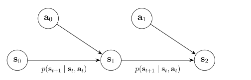
The basic picture is simple. At time $t$, the agent is in some current state $s_t$. It chooses an action $a_t$, and then the world moves to a next state $s_{t+1}$.

For example, consider chess. The current state is the board position, and the action is the move chosen by the player. After the move is made, the next state is the new board position.

Driving can also be viewed in the same way. The current state is the road situation around the car: where the car is, how it is moving, and what is happening nearby. The action might be to accelerate, brake, or steer. After that action, the next state is the road situation a moment later.

We call the rule that describes this change the transition model, or dynamics model:

$$p(s_{t+1} \mid s_t, a_t)$$

This notation means that, given $s_t$ and $a_t$, the model assigns probabilities to possible next states $s_{t+1}$.

In chess, this rule is just the rules of the game. Given a board position and a legal move, the next board position is fixed. So chess has deterministic and known dynamics.

In driving, this rule is much harder to write down. The next road situation depends on the car, the road, and other drivers. The same action in a similar-looking situation may not always give the same result. So driving has stochastic and unknown dynamics.

The key assumption in an MDP is the Markov property. It says that the next state only depends on the current state and action, not on the full history before them:

$$p(s_{t+1} \mid s_t, a_t, s_{t-1}, a_{t-1}, \ldots) = p(s_{t+1} \mid s_t, a_t)$$

There is one thing to be careful about. The Markov property does not mean the past is useless. It means that the state $s_t$ should already contain the relevant information from the past. If important information is missing from the state, then the process may no longer look Markov.

The Reinforcement Learning Objective

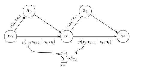
The dynamics model describes how the environment responds to an action. It tells us how the state changes after the agent acts.

What the agent can control is which action to choose in the current state. We call this rule the policy, usually written as $\pi$.

For example, in chess, the policy tells the player which move to make from the current board position. In driving, the policy tells the car whether to accelerate, brake, or steer from the current road situation.

If the policy is stochastic, we write it as

$$\pi(a_t \mid s_t)$$

which means the probability of choosing action $a_t$ in state $s_t$.

Now we need a way to say whether a policy is good or bad. For this, we add rewards to the MDP. A reward is a number that tells the agent how desirable an outcome is.

In chess, the reward might be positive for winning and negative for losing. In driving, the reward might encourage safe progress and penalize collisions or leaving the lane.

At each time step, the agent is in state $s_t$, chooses action $a_t$ using its policy, receives reward $r_t$, and moves to the next state $s_{t+1}$. More generally, the reward and next state can be sampled from the dynamics:

$$(r_t, s_{t+1}) \sim p(\cdot \mid s_t, a_t)$$

If the reward is deterministic, we can write it as a reward function $r(s_t, a_t)$.

Once a policy is fixed, the policy and the dynamics together define a distribution over trajectories. One trajectory can be written as

$$\tau = (s_0, a_0, r_0, s_1, a_1, r_1, \ldots, s_T)$$

Here, the initial state $s_0$ is sampled from the initial state distribution $p_0$. Following the MDP, the probability of a trajectory under policy $\pi$ is

$$p_\pi(\tau) = p_0(s_0) \prod_{t=0}^{T-1} \pi(a_t \mid s_t) p(r_t, s_{t+1} \mid s_t, a_t)$$

Now we can define the reinforcement learning objective. A policy is good if the trajectories it generates tend to have high total reward. Usually, we write this as maximizing the expected discounted sum of rewards:

$$\max_\pi \mathbb{E}_{\tau \sim p_\pi(\tau)} \left[ \sum_{t=0}^{T-1} \gamma^t r_t \right]$$

The factor $\gamma$ appears because we often want the return to be well-defined even when the trajectory is very long or infinite. If we simply sum rewards forever, the total reward may diverge. When rewards are bounded and $\gamma < 1$, the discounted sum is finite:

$$\sum_{t=0}^{\infty} \gamma^t r_t$$

Most RL algorithms assume $\gamma < 1$ for mathematical convenience. In practice, if the undiscounted total reward is already well bounded, using $\gamma = 1$ is usually fine.

When Does an MDP End?

In the trajectory notation above, we wrote the final time as $T$. So how is $T$ determined?

In general, $T$ is not a pre-determined, fixed value. An MDP ends when the trajectory reaches a terminal state. For example, in chess, the game ends when the board reaches a terminal state, such as checkmate or draw. We can write this terminal state as $s_{\mathrm{term}}$:

$$s_T = s_{\mathrm{term}}$$

So $T$ is the time when the trajectory ends.

One thing to notice is that $T$ is a random variable, which makes it inconvenient to work with mathematically. For example, we should not casually write

$$\mathbb{E}_{\tau \sim p_\pi(\tau)} \left[ \sum_{t=0}^{T} r_t \right] = \sum_{t=0}^{T} \mathbb{E}_{\tau \sim p_\pi(\tau)}[r_t]$$

because the upper limit still depends on the sampled trajectory.

A common trick is to define an equivalent MDP that never formally stops. We make the terminal state absorbing: once the process reaches $s_{\mathrm{term}}$, it stays there forever and receives zero reward:

$$p(r_t = 0, s_{t+1} = s_{\mathrm{term}} \mid s_t = s_{\mathrm{term}}, a_t) = 1$$

After this transformation, the policy at $s_{\mathrm{term}}$ does not matter. No matter what action is chosen, the process stays in the terminal state and receives no further reward. This lets us use infinite-horizon notation while still representing tasks that end.

Partially Observable MDP

So far, we have assumed that the agent can observe the full state $s_t$. In many problems, this is not true. The agent only receives an observation $o_t$, which may contain only partial information about the true state.

For example, in driving, the full state would include everything relevant in the environment. But the car only observes what its sensors can measure. If another car is hidden behind a truck, that information is part of the true state, but it may not appear in the current observation.

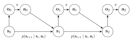
This setting is called a partially observable MDP, or POMDP. In a POMDP, the policy is usually written as a function of the observation:

$$\pi(a_t \mid o_t)$$

instead of the full state $s_t$.

For the rest of this post, I will assume a fully observable MDP. In many cases, the same ideas can be adapted to POMDPs by replacing the state with the observation.

Stationarity

One more assumption in this post is that the dynamics are stationary. This means the transition model does not change over time:

$$p_t(r_t, s_{t+1} \mid s_t, a_t) = p(r_t, s_{t+1} \mid s_t, a_t)$$

So the same state and action follow the same dynamics at every time step.

If the dynamics change with time, they are non-stationary. One example is the fixed-horizon case, where the episode is forced to end at a pre-determined time $T$. This is different from the terminal-state view above, where $T$ depends on the trajectory. In the fixed-horizon case, the transition rule depends on time:

$$\begin{aligned} p_{T-1}(s_T = s_{\mathrm{term}} \mid s_{T-1}, a_{T-1}) &= 1 \\ p_t(s_{t+1} = s_{\mathrm{term}} \mid s_t, a_t) &= 0, \qquad t = 0,\ldots,T-2 \end{aligned}$$

When dynamics are non-stationary, the optimal policy may also need to depend on time. Instead of writing

$$\pi(a_t \mid s_t)$$

we may need to write

$$\pi_t(a_t \mid s_t)$$

For the rest of this post, I will assume stationary dynamics.

Value Functions

Let us define a few useful functions for working with a policy $\pi$.

The state value function $V^\pi$ measures the expected return starting from state $s$ and then following policy $\pi$:

$$V^\pi(s) = \mathbb{E}_{\tau \sim p_\pi(\tau \mid s_0 = s)} \left[ \sum_{t=0}^{T-1} \gamma^t r_t \right]$$

The state-action value function $Q^\pi$ measures the expected return starting from state $s$, first taking action $a$, and then following policy $\pi$:

$$Q^\pi(s,a) = \mathbb{E}_{\tau \sim p_\pi(\tau \mid s_0 = s, a_0 = a)} \left[ \sum_{t=0}^{T-1} \gamma^t r_t \right]$$

So $V^\pi(s)$ tells us how good it is to be in a state under policy $\pi$, while $Q^\pi(s,a)$ tells us how good it is to first take action $a$ from that state and then follow $\pi$.

The advantage function compares these two quantities:

$$A^\pi(s,a)=Q^\pi(s,a)-V^\pi(s).$$

The advantage tells us whether action $a$ is better or worse than the average action under policy $\pi$ at state $s$. If $A^\pi(s,a)>0$, then action $a$ is better than average. If $A^\pi(s,a)<0$, then it is worse than average.

Basic Properties of $V^\pi$ and $Q^\pi$

The relationship between $V^\pi$ and $Q^\pi$ follows directly from the way an MDP generates a trajectory.

If we start from state $s$, the policy first chooses an action $a \sim \pi(\cdot \mid s)$. After that, the expected return is $Q^\pi(s,a)$. Therefore, the value of state $s$ is the average state-action value under the policy:

$$V^\pi(s) = \mathbb{E}_{a \sim \pi(\cdot \mid s)} \left[ Q^\pi(s,a) \right]$$

Conversely, suppose we start from state $s$ and first take action $a$. The environment gives reward $r$ and next state $s'$. From that point on, we follow policy $\pi$, so the remaining expected return is $V^\pi(s')$. Therefore,

$$Q^\pi(s,a) = \mathbb{E}_{(r,s') \sim p(\cdot \mid s,a)} \left[ r + \gamma V^\pi(s') \right]$$

These two equations connect $V^\pi$ and $Q^\pi$. Combining them gives the one-step transition property.

For the state value function,

$$V^\pi(s) = \mathbb{E}_{a \sim \pi(\cdot \mid s),\ (r,s') \sim p(\cdot \mid s,a)} \left[ r + \gamma V^\pi(s') \right]$$

For the state-action value function,

$$Q^\pi(s,a) = \mathbb{E}_{(r,s') \sim p(\cdot \mid s,a),\ a' \sim \pi(\cdot \mid s')} \left[ r + \gamma Q^\pi(s',a') \right]$$

Bellman Equation and Bellman Operator

For a fixed policy $\pi$, define the Bellman operator $T^\pi$ as the operator that maps $V:\mathcal{S}\to\mathbb{R}$ to $T^\pi V:\mathcal{S}\to\mathbb{R}$:

$$(T^\pi V)(s) = \mathbb{E}_{a \sim \pi(\cdot \mid s),\ (r,s') \sim p(\cdot \mid s,a)} \left[ r + \gamma V(s') \right]$$

The one-step transition property for $V^\pi$ can then be written as

$$T^\pi V^\pi = V^\pi.$$

So $V^\pi$ is a fixed point of the Bellman operator. The important fact is that the converse also holds: if a bounded function satisfies this fixed point equation, then it must be the true value function $V^\pi$.

Theorem. Let $\pi$ be a fixed policy. Assume $\gamma \in (0,1)$, $|\mathcal{S}|<\infty$, and $|r|\le R<\infty$ almost surely. Then $V^\pi$ exists and satisfies the Bellman equation

$$T^\pi V^\pi = V^\pi.$$

Conversely, if a bounded function $V:\mathcal{S}\to\mathbb{R}$ satisfies

$$T^\pi V = V,$$

then $V=V^\pi$.

Moreover, if we start from any bounded initial function $V_0$ and repeatedly apply the Bellman operator, the result converges to $V^\pi$:

$$\lim_{k\to\infty} \left\| (T^\pi)^k V_0 - V^\pi \right\|_\infty = 0.$$

Proof

Since rewards are bounded and $\gamma \in (0,1)$, the discounted return is bounded, so $V^\pi$ is well defined. Also, by the one-step transition property, $T^\pi V^\pi = V^\pi$. Thus $V^\pi$ is a fixed point of $T^\pi$.

Now we show that this fixed point is unique. We will use the Banach fixed point theorem.

Banach fixed point theorem. Let $(\mathcal{X}, d)$ be a complete metric space. Suppose $T:\mathcal{X}\to\mathcal{X}$ is a $\gamma$-contraction with $\gamma < 1$, meaning

$$d(Tx, Ty) \le \gamma d(x,y) \quad \forall x,y \in \mathcal{X}.$$

Then $T$ has a unique fixed point $x^*$. Moreover, for any $x\in\mathcal{X}$,

$$T^k x \to x^* \quad \text{as } k\to\infty.$$

We will apply this theorem to the Bellman operator. Here, we work with bounded functions $V:\mathcal{S}\to\mathbb{R}$ under the sup norm

$$\|V\|_\infty = \max_s |V(s)|.$$

For any two bounded functions $V_1,V_2:\mathcal{S}\to\mathbb{R}$,

$$\begin{aligned} \|T^\pi V_1 - T^\pi V_2\|_\infty &= \max_s \left| (T^\pi V_1)(s) - (T^\pi V_2)(s) \right| \\ &= \max_s \left| \mathbb{E}_{a \sim \pi(\cdot \mid s),\ (r,s') \sim p(\cdot \mid s,a)} \left[ \gamma \left(V_1(s') - V_2(s')\right) \right] \right| \\ &\le \gamma \max_s \mathbb{E}_{a \sim \pi(\cdot \mid s),\ (r,s') \sim p(\cdot \mid s,a)} \left[ \left|V_1(s') - V_2(s')\right| \right] \\ &\le \gamma \|V_1 - V_2\|_\infty. \end{aligned}$$

Therefore, $T^\pi$ is a $\gamma$-contraction. By the Banach fixed point theorem, $T^\pi$ has a unique fixed point, and repeatedly applying $T^\pi$ from any bounded initial function $V_0$ converges to that fixed point.

Since $V^\pi$ is already a fixed point, it must be the unique fixed point. Therefore, if any bounded function $V$ satisfies $T^\pi V=V$, then $V=V^\pi$. Also,

$$\lim_{k\to\infty} \left\| (T^\pi)^k V_0 - V^\pi \right\|_\infty = 0.$$

The same idea holds for the state-action value function $Q^\pi$. Define the Bellman operator on $Q:\mathcal{S}\times\mathcal{A}\to\mathbb{R}$ by

$$(T^\pi Q)(s,a) = \mathbb{E}_{(r,s') \sim p(\cdot \mid s,a),\ a' \sim \pi(\cdot \mid s')} \left[ r + \gamma Q(s',a') \right]$$

Theorem. Let $\pi$ be a fixed policy. Assume $\gamma \in (0,1)$, $|\mathcal{S}|<\infty$, $|\mathcal{A}|<\infty$, and $|r|\le R<\infty$ almost surely. Then $Q^\pi$ exists and satisfies the Bellman equation

$$T^\pi Q^\pi = Q^\pi.$$

Conversely, if a bounded function $Q:\mathcal{S}\times\mathcal{A}\to\mathbb{R}$ satisfies

$$T^\pi Q = Q,$$

then $Q=Q^\pi$.

Moreover, if we start from any bounded initial function $Q_0$ and repeatedly apply the Bellman operator, the result converges to $Q^\pi$:

$$\lim_{k\to\infty} \left\| (T^\pi)^k Q_0 - Q^\pi \right\|_\infty = 0.$$

The proof is almost identical to the proof for $V^\pi$. The same contraction argument applies, now using the sup norm over state-action pairs.

---

This is the end of the first post. We introduced the basic setup of reinforcement learning: MDPs, rewards, policies, trajectories, value functions, and Bellman equations. In the next post, we will look at how to optimize the policy.